One of the main concepts studied in the field of differential calculus is based on the notion of change - specifically, how one quantity changes compared to another. Perhaps a more succinct version of this physical definition would be "rate of change." Alternately, a geometric definition could simply be the slope of a curve at a particular point. The underlying key to this branch of mathematics is the concept of the
derivative. In this post, I will introduce various aspects of the derivative - please click the Facebook Like button if this is helpful for you!
First, let's consider the derivative in terms of rate of change. And to do that, let's talk about velocity. We know that velocity is equal to
distance per unit time. However, that is a very general description of it. If you drive from your home to the grocery store on the other side of town, you can do the math by dividing your total distance travelled by the time it took you to get there, but what does this number tell you? It actually tells you the
average velocity of your trip. Think about it. You had to stop for red lights, stop signs, pedestrians. Maybe you sped up to pass a slow driver. Don't forget about the actual acceleration of your car from a standstill, and then the deceleration whenever you needed to stop. All of this factors into the calculation of your average velocity, which is simply how far you go in a measured amount of time.
Now, let's consider how to calculate the average velocity of your car between your home and the first stop sign, while on your way to the grocery store. You no longer have several stops to deal with. You get in your car, accelerate, then as you approach the stop sign, you decelerate to a stop. Your average velocity is calculated from a much shorter interval, and will have much less variation to it. So, your average velocity will be more representative of your actual velocity at any given time.
To extend this demonstration even further, let's consider the small portion of your trip that is measured between two street lights 10 meters apart that you pass while you are in full motion. That is, let's assume that we want to measure the velocity without having to calculate stop signs, etc. Our time interval for the measurement is much smaller, and calculating the velocity by dividing the distance by the time it takes to go from one light to the other is even more representative of your velocity at any point between them.
What I am trying to demonstrate is the concept of
instantaneous velocity. If you shrink down your time interval of measurement infinitesimally, the two time points approach each other at a single point, and so the
average velocity between the two super close points approaches the
instantaneous velocity of the single point.
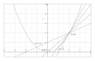
Graphically, this is essentially the same thing you do when you calculate the slope of a tangent line to a curve. You pick two lines on the curve and calculate the slope of the line between them, and then you
use limits to make the points get closer and closer together until they are almost the same, and the slope of the line connecting those two infinitely close points is the tangent. (Check out my previous post about using limits to find tangents if you'd like a refresher of this topic:
http://sk19math.blogspot.ca/2012/06/using-limits-to-find-tangents.html)
Because this type of limit occurs so frequently in maths, science, and engineering, it is given the special name of "
derivative," and you calculate derivatives through the process of "
differentiation." So, one interpretation of the derivative is an expression of the instantaneous rate of change (velocity) at a particular point on the curve - a large derivative corresponds to a high rate of change (a steep curve), and conversely a small derivative corresponds to a low rate of change (a relatively flat curve). As a specific example, if you actually have a graph of position (displacement) of an object vs. time, the derivative of the curve at any time point represents the velocity of that object at that specific time. This may take a little practice to become comfortable with the concept, but suffice it to say at this point that learning how to use derivatives is incredibly important to be able to work out more complex concepts relatively easily.
Let's look at this now in the more formal terms of mathematical symbols and equations. Consider any curve y = f(x).
Now, let us identify the point P on the curve f(x) for when x = a. That is to say, the point (a, f(a)).
Now, let's go a step further, and identify a point Q that is h units away from a on the x-axis. If it is h units away from a, we can call it "a + h". (If this is confusing, think about it with numbers instead. Start at, say, x = 3 (instead of a). Now we want to know what is going on 5 units (instead of h) away from x = 3. In other words, we have 3, and we have 3 + 5.) As such, we can therefore identify a point Q ((a + h), f(a + h)).
Now that we have two arbitrary points, let's determine the slope of the straight line that would connect the two. We can use the same slope formula that we always use, slope = rise/run, but substitute in our variables that we identified above. So, we have:
Now, imagine that the distance h between the two points is getting smaller and smaller. Or in other words, consider the case of when h approaches 0. By doing this, we calculate the slope of the line connecting two infinitesimally close points - which means that we are actually approaching the slope of the tangent line to the curve at point a. In this case, we would express this slope as a limit in the following way, which actually corresponds to the definition of the derivative of a function f at a number a. The derivative is given the special symbol f'(x), and we say "f prime x", and we express it like this:
Another way of expressing this can be found if we recognize that a + h is really just any x value. So, we can say x = a + h (and by extension, h = x - a), and modify the above derivative definition accordingly:
With this modified equation, it actually becomes a matter of arithmetic to determine the slope at a point. Here is an example of a kind of question that you will see:
"Find the derivative (or, determine the slope of the tangent) of the function f(x) = x2 - 4 at a number a."
To do this, write the provided equation into the definition, and reduce until you have an answer. Notice below how I combine terms and recognize the identity of a difference of squares.
What this final result tells you is that for our curve, f(x)
= x2 - 4, at any number a along it, the slope of the tangent (AKA, the derivative at that point) is equal to the term 2a. Graph it out and try with several values to convince yourself that it's true! Consider when x = 5. You can determine from the original equation that we have the point (5, 21). At this point on the curve, the slope of the tangent equals 2 x 5 = 10.
Going back to the definition of the derivative that I gave above, you can also apply the
concept of point-slope form to it to get a different way of seeing it. Letting y = f(x), you can rearrange the definition as follows, by simple reorganization of the terms:

Here's a more visual exercise that you may soon encounter.
"If you are provided a graph of a function f(x) - not necessarily the equation - sketch out what the graph of the derivative f'(x) would look like."
When you actually have the numbers and equation, this becomes much easier... assuming you know how to easily recognize derivatives from the original equations. However, if provided ONLY the picture of the curve, this becomes a bit more abstract, but not really that challenging. It DOES require you to understand the concept of derivatives and rate of change though. Here is why. Take some random curve that you can draw. Any curve will do for this exercise:
The key is
rate of change. We have seen that slope is equal to rate of change, so we want to pay particular attention to the slope at several points. And the easiest points to notice are those where the slope is equal to 0. These are all the peaks and valleys of the curve. What I have done next is highlight with red bars all of the zero-slopes:

Now, to proceed with sketching the graph of the derivative f'(x) vs x, you can start by plotting the points where f'(x) is equal to zero. From there you can then go on to say where the curve of f(x) has a positive, increasing slope, and then sketch that into your f'(x) graph accordingly. Similarly, decreasing slopes on the f(x) curve will be negative values on the f'(x) curve. For the sake of this exercise, don't worry so much about how high or low the slopes are. Just focus on whether they are positive or negative at the various parts of the graph. I have gone ahead and plotted out the actual curve of the derivative below in green, alongside the original curve of f(x). You can see that the f'(x) curve crosses zero wherever the curve for f(x) has peaks or valleys, and the steeper the f(x) curve, the more extreme the f'(x) curve at that same point.

Of course, having a mathematical definition wouldn't be any fun if there were no conditions or rules associated with it - and the definition of derivatives is no exception. One such rule states that a function is differentiable at a point
a if the derivative f'(a) exists. Seems intuitive enough. If a derivative at a point exists, then the base function is differentiable at that point. Probably one of those rules that doesn't really even need to be said. :)
I'm not going to graph this one out, but it is for you to think on.
Consider the case of f(x) = |x|. Where is it differentiable?
If you consider the derivative of the left hand side, it equals -1. The f'(x) on the right hand side is 1. This function then is obviously differentiable when x < 0, and when x > 0. But what about when x = 0? In this case, since the right hand limit approaches 1 as x approaches 0 from the right, and the left hand limit approaches -1 as x approaches 0 from the left, one must conclude that f'(0) does not exist because
both of the one-sided limits approach different numbers.
An extension of this example actually describes a second rule for limits: if f'(a) exists, then the function f(x) is
continuous as
a. Recall that
continuity of a curve is based on the notion that as you approach a point from both the left and the right, the limit of each side approaches the same value. In the example above, approaching 0 from either side resulted in different limits, and hence the graph is not continuous at 0.
Keep this in mind as you see various graphs of functions. Curves that have a sharp point will not be differentiable at the point, for the reason given above. Similarly, discontinuous curves (i.e. curves with gaps in them) will not have a derivative at the break point either because the one-sided limits do not agree. If f(x) is not continuous as point
a, then f'(a) does not exist. A third condition to watch out for is where a graph has a vertical tangent line, in which case the slope is infinite.
Now, I'm going to wrap up this mammoth of a maths post with something a bit easier to talk about:
notation of derivatives. I have already described a few ways to express these values. I talked about expressing them as limits, and using infinitesimally smaller intervals, and that is a good way to work through them. Symbolically, I said that you can write f'(x) to denote the derivative of the functions f(x). This will likely be the easiest way for you to use it and to recognize it, though here are a few others that mean the same thing:
Each of these terms means the exact same thing. In particular, the D and d/dx are specifically called the
differentiation operators, and you can see they have a few variations. Similarly, dy/dx is symbolic of derivatives for historical reasons. Read up on
Gottfried Wilhelm Leibniz to learn more about the origins of calculus, where you will see that he introduced this way of representing it. Sometimes, you may see dy/dx referred to as "Leibniz notation."
And with that final tidbit of mathematical goodness, I am going to end this post. I intend to follow this with another post in the near future that introduces differentiation methods and strategies.
Much like the exponent rules, there are also several differentiation rules, and I hope to be able to explain them for you as well. If you have made it to this point of my post, thanks for reading, and please be sure to click the Facebook Like button below or at the top, and I'd appreciate a Google +1 as well below if this was helpful!

 Here's a better way to remember this, which may be even easier to think of but harder to draw: imagine that the exponent is a pile of sequential number cards (e.g. 1, 2, 3, 4, 5...) with the high card on top. When you have to find the derivative, take the top card and place it in front of the x, leaving the card beneath it (which is 1 number smaller) visible. It's easier to actually do this than to draw it, but it's a great way to remember this formula because it is so easy to visualize!


+derivatives.jpg)
+a+h.jpg)


